R語言與抽樣技術學習筆記（bootstrap）-CDA數據分析師官網

熱線電話：13121318867

登錄

R語言與抽樣技術學習筆記（bootstrap）

2017-07-20

R語言與抽樣技術學習筆記（bootstrap）

Bootstrap方法

Bootstrap一詞來源于西方神話故事“The adventures of Baron Munchausen”歸結出的短語“to pull oneself up by one's bootstrap"，意味著不靠外界力量，依靠自身提升性能。
　　Bootstrap的基本思想是：因為觀測樣本包含了潛在樣本的全部的信息，那么我們不妨就把這個樣本看做“總體”。那么相關的統計工作（估計或者檢驗）的統計量的分布可以從“總體”中利用Monte Carlo模擬得到。其做法可以簡單地概括為：既然樣本是抽出來的，那我何不從樣本中再抽樣。

bootstrap基本方法

1、采用重抽樣技術從原始樣本中抽取一定數量（自己給定）的樣本，此過程允許重復抽樣。
　　2、根據抽出的樣本計算給定的統計量T。
　　3、重復上述N次（一般大于1000），得到N個統計量T。其均值可以視作統計量T的估計。
　　4、計算上述N個統計量T的樣本方差，得到統計量的方差。
　　上述的估計我們可以看成是Bootstrap的非參數估計形式，它基本的思想是用頻率分布直方圖來估計概率分布。當然Bootstrap也有參數形式，在已知分布下，我們可以先利用總體樣本估計出對應參數，再利用估計出的分布做Monte Carlo模擬，得到統計量分布的推斷。
　　值得一提的是，參數化的Bootstrap方法雖然不夠穩健，但是對于不平滑的函數，參數方法往往要比非參數辦法好，當然這是基于你對樣本的分布有一個初步了解的基礎上的。
　　例如：我們要考慮均勻分布U(θ)的參數θ的估計。我們采用似然估計。

    data.sim <- runif(10)
    theta.hat <- max(data.sim)
    theta.boot1 <- replicate(1000, expr = {
        y <- sample(data.sim, size = 10, replace = TRUE)
        max(y)
    })

    theta.boot1.estimate <- mean(theta.boot1)
    cat("the original estimate is ", theta.hat, "after bootstrap is ", theta.boot1.estimate)

## the original estimate is 0.7398 after bootstrap is 0.7138

[plain] view plain copy
print?

    hist(theta.boot1)

從結果來看，倒不是說估計有多不好，只是說方差比較大，而且它的經驗分布真的不太像真正的分布，這個近似很糟糕，導致的直接結果是方差也很大。
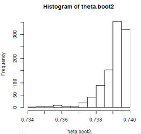
　　如果采用參數方法，我們再來看看：

    theta.boot2 <- replicate(1000, expr = {
        y <- runif(1000, 0, theta.hat)
        max(y)
    })

    theta.boot2.estimate <- mean(theta.boot2)
    cat("the original estimate is ", theta.hat, "after bootstrap is ", theta.boot2.estimate)

## the original estimate is 0.7398 after bootstrap is 0.7391

[plain] view plain copy
print?

    hist(theta.boot2)

結果從直方圖來看是更優秀了，估計也更好一些，關鍵是方差變小了，從非參數的0.0402減少到了7.3944 × 10-4。

bootstrap推斷與bootstrap置信區間

既然我們已經得到了Bootstrap估計量的經驗分布函數，那么一個自然的結果就是我們可以利用這個分布對統計量做出一些統計推斷。例如可以推測估計量的方差，估計量的偏差，估計量的置信區間等。
現在，我們就來考慮如何做Bootstrap的統計推斷。

利用Bootstrap估計偏差

既然Bootstrap將獲得的樣本樣本看成了”總體“，那么估計量T自然是一個無偏的估計，Bootstrap數據集構造的”樣本“的統計量T與原始估計量T的偏差自然就是估計量偏差的一個很好的估計。
　　具體做法是：
1. 從原始樣本x1,?,xn中有放回的抽取n個樣本構成一個Bootstrap數據集，重復這個過程m次，得到m個數據集。
2. 對于每個Bootstrap數據集，計算估計量T的值，記為T?j。
3.T?j的均值是T的無偏估計，而其與T的差是偏差的估計。

利用Bootstrap估計方差

估計量T的方差的估計可以看做每個Bootstrap數據集的統計量T的值的方差。
　　以我們遺留的問題，求1到100中隨機抽取10個數的中位數的方差為例來說明。

n <- 10
    x <- sample(1:100, size = n)
    Mboot <- replicate(1000, expr = {
        y <- sample(x, size = n, replace = TRUE)
        median(y)
    })
    print(var(Mboot))

## [1] 334.2

這個應該是一個正確的估計了。Efron指出要得到標準差的估計并不需要非常多的Bootstrap數據集（m不需要過分的大），通常50已經不錯了，m>200是比較少見的（區間估計可能需要多一些）
　　在R中，bootstrap包的函數bootstrap可以幫助你完成這一過程。bootstrap函數的調用格式如下：

bootstrap(x,nboot,theta,…, func=NULL)　　

參數說明：

x：原始抽樣數據　　

theta：統計量T　　

nboot：構造Bootstrap數據集個數

library(bootstrap)
    theta <- function(x) {
        median(x)
    }
    results <- bootstrap(x, 100, theta)
    print(var(results$thetastar))

## [1] 393.2

可以看到兩個的結果是相近的，所以，利用這個函數還是不錯的選擇。類似的還有boot包的boot函數。我們在相關數據的Bootstrap推斷中會用到。

相關數據的Bootstrap推斷

回歸數據的Bootstrap推斷

我們之所以可以采用Bootstrap去做這些估計，蘊含了一個很重要的假設，這些樣本是近似iid的，然而我們不能保證需要推斷的數據都是近似獨立同分布的，對于相關數據的Bootstrap推斷，我們常用的方法有配對的Bootstrap（paired Bootstrap）與殘差法。
　　先說paired Bootstrap，它的基本想法是，對于觀測構成的數據框，雖然觀測的每一行數據是相關的，但是每行是獨立的，我們Bootstrap抽樣，每次抽取一行，而不是單獨的抽一個數即可。
例如，數據集women列出了美國女性的平均身高與體重，我們以體重為響應變量，身高為協變量進行回歸，得到回歸系數的估計。
　　使用paired Bootstrap：

m <- 200
n <- nrow(women)
beta <- numeric(m)
for (b in 1:m) {
    i <- sample(1:n, size = n, replace = TRUE)
    weight <- women$weight[i]
    height <- women$height[i]
    beta[b] <- lm(weight ~ height)$coef[2]
}
cat("the estimate of beta is", lm(weight ~ height, data = women)$coef[2], "paired bootstrap estimate is",
    mean(beta))

## the estimate of beta is 3.45 paired bootstrap estimate is 3.452

cat("the bias is", lm(weight ~ height, data = women)$coef[2] - mean(beta), "the stand error is",
sd(beta))

## the bias is -0.002468 the stand error is 0.126

我們可以看到，估計量是無偏的，但是這個辦法估計的方差變化較小，可能導致區間估計是不夠穩健。我們可以利用boot包的boot函數來解決。

beta <- function(x, i) {
xi <- x[i, ]
coef(lm(xi[, 2] ~ xi[, 1]))[2]
}
library(boot)
obj <- boot(data = women, statistic = beta, R = 2000)
obj

##
## ORDINARY NONPARAMETRIC BOOTSTRAP
##
##
## Call:
## boot(data = women, statistic = beta, R = 2000)
##
##
## Bootstrap Statistics :
## original bias std. error
## t1* 3.45 -0.002534 0.1208

接下來我們說說殘差法：
1. 由觀測數據擬合模型.
2. 獲得響應y^i與殘差?i
3. 從殘差數據集中有放回的抽取殘差，構成Bootstrap殘差數據集?^i（這是近似獨立的）
4. 構造偽響應Y?i=yi+?^i
5. 對x回歸偽響應Y，得到希望得到的統計量，重復多次，得到希望的統計量的經驗分布，利用它做統計推斷
　　我們將women數據集的例子利用殘差法在做一次，R代碼如下：

lm.reg <- lm(weight ~ height, data = women)
    y.fit <- predict(lm.reg)
    y.res <- residuals(lm.reg)
    y.bootstrap <- rep(1, 15)
    beta <- NULL
    for (p in 1:100) {
        for (i in 1:15) {
            res <- sample(y.res, 1, replace = TRUE)
            y.bootstrap[i] <- y.fit[i] + res
        }
        beta[p] <- lm(y.bootstrap ~ women$height)$coef[2]
    }
    cat("the estimate of beta is", lm(weight ~ height, data = women)$coef[2], "paired bootstrap estimate is",
        mean(beta))

## the estimate of beta is 3.45 paired bootstrap estimate is 3.436

cat("the bias is", lm(weight ~ height, data = women)$coef[2] - mean(beta), "the stand error is",
sd(beta))

## the bias is 0.01436 the stand error is 0.08561

可以看到，利用殘差法得到的方差更為穩健，做出的估計也更為的合理。
　　這里需要指出一點，Bootstrap雖然可以處理相關數據，但是在變量篩選方面，其效果遠不如Cross Validation準則好。

時間序列數據中的Bootstrap方法

還有一類數據的相關性是上述假定也不滿足的，那就是時間序列數列。那么如何利用Bootstrap來推斷時間序列呢？我們以1947年–1991年美國GNP季度增長率數據為例進行說明。這個數據來自《金融時間序列分析》一書，數據可以在這里下載。
我們先來了解一下這個數據：

data <- read.table("D:/R/data/dgnp82.txt")
gnp <- data * 100
gnp1 <- ts(gnp, fre = 4, start = c(1947, 2))
par(mfrow = c(3, 1))
plot(gnp1, type = "l")
acf(gnp1, lag = 24)
pacf(gnp1, lag = 24)

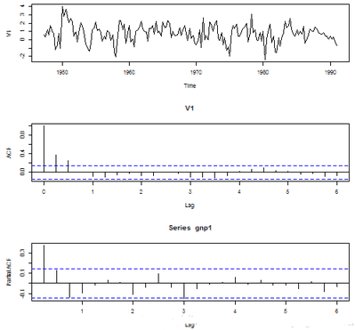
對于這個數據集，假設我想利用這些增長率估計平均增長率，顯然直接從這些數據中有放回抽樣是不合理的，因為它們是相依的，按照金融的說法，它們還存在波動性聚集。但是我們仍然不妨先這么計算，可以與之后的“正確”結果對比一下。

## mean estimate is: 0.7691 variance is: 0.01215

對于這類問題，一個利用我們前面描述的辦法可以解決的方案就是利用參數的Bootstrap方法。我們可以先考慮對時間序列建模：

library(tseries)
adf.test(gnp1)

##
## Augmented Dickey-Fuller Test
##
## data: gnp1
## Dickey-Fuller = -5.153, Lag order = 5, p-value = 0.01
## alternative hypothesis: stationary

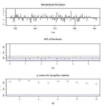
我們從上面的圖片以及平穩性檢驗很快就可以發現，AR(3)是對這個時間序列的不錯的描述，那么我們先求取這個模型的參數估計：

model <- arima(gnp1, order = c(3, 0, 0))
tsdiag(model)

那么我們的參數Bootstrap可以這么做：

simu <- function(model) {
        n <- 1000 # Generate AR(3) process
        a <- as.numeric(coef(model))
        e <- rnorm(n + 200, 0, sqrt(9.48e-05))
        x <- double(n + 200)
        x[1:3] <- rnorm(3)
        for (i in 4:(n + 100)) {
            x[i] <- a[1] * x[i - 1] + a[2] * x[i - 2] + a[3] * x[i - 3] + a[4] +
                e[i]
        }
        x <- ts(x[-(1:200)])
        mean(x)
    }
    mean.boot1 <- replicate(1000, expr = simu(model))
    cat("mean estimate is:", (mean.boot.estimate <- mean(mean.boot)), "variance is:",
        var(mean.boot))

## mean estimate is: 0.7691 variance is: 0.01215

可以看到兩者的結果是差不多的，究其原因是因為這是一個平穩過程，所以相差不大，我們來看一個非平穩的例子，很快就能發現不同：

data.sim <- arima.sim(list(order = c(2, 2, 0), ar = c(0.7, 0.2)), n = 500)
cat("mean is:", mean(data.sim))

## mean is: -5574## [1] "In the iid case:"

mean.boot <- replicate(1000, expr = {
        y <- sample(data.sim, size = 2 * length(data.sim), replace = TRUE)
        mean(y)
    })
    cat("mean estimate is:", (mean.boot.estimate <- mean(mean.boot)), "variance is:",
        var(mean.boot))

## mean estimate is: -5560 variance is: 86089## [1] "In the dependence case:"

model <- arima(data.sim, order = c(2, 2, 0))
    simu <- function(model) {
        x <- arima.sim(list(order = c(2, 2, 0), ar = as.numeric(coef(model))), n = 500)
        mean(x)
    }
    mean.boot1 <- replicate(1000, expr = simu(model))
    cat("mean estimate is:", (mean.boot.estimate <- mean(mean.boot)), "variance is:",
        var(mean.boot))

## mean estimate is: -5560 variance is: 86089

但是這種明顯需要知道模型，或者正確模型設定才能得到比較好的結果的Bootstrap是不穩健的，如果上面我們采用了一個非真實的模型，結果會變為：

(model <- arima(data.sim, order = c(5, 3, 1)))

##
## Call:
## arima(x = data.sim, order = c(5, 3, 1))
##
## Coefficients:
##          ar1     ar2     ar3     ar4     ar5    ma1
##       -1.149 -0.260 -0.137 -0.142 -0.024 0.897
## s.e.   0.121   0.074   0.069   0.070   0.048 0.112
##
## sigma^2 estimated as 1.02: log likelihood = -713.5, aic = 1441

從建模的角度來說，這個也是不錯的一個模型，那么它的估計可以由下面代碼給出：

simu <- function(model) {
        x <- arima.sim(list(order = c(5, 3, 1), ar = as.numeric(coef(model))[1:5],
            ma = as.numeric(coef(model))[6]), n = 500, sd = sqrt(1.067))
        mean(x)
    }
    mean.boot1 <- replicate(1000, expr = simu(model))
    cat("mean estimate is:", (mean.boot.estimate <- mean(mean.boot)), "variance is:",
        var(mean.boot))

## mean estimate is: -5560 variance is: 86089

我們可以想見，在置信區間上這會給出一個比較寬的置信區間，這很有可能是我們不想見到的。那么，我們有沒有穩健些的非參數方法呢？這是有的，這個方法通常被稱為“Block Bootstrap”方法。
　　Block Bootstrap的思想很簡單，雖然時間序列存在相關，但是自相關系數可能在若干延遲后就可以忽略不計了。那么我們取一個區間長度，將整個樣本分為若干個區間，序列的順序不改變，而區間之間看做近似獨立的，我們對這些區間（block）做Bootstrap。如果區間間不存在重疊，我們稱之為"Nonmoving block bootstrap";如果區間存在重疊（如樣本為1, 2, 3, 4, 5, 6, 7, 8, 9, 10，我們將區間分為就可以稱作"Moving block bootstrap"。
　　我們還是來考慮GNP數據，我們假設block長度為6，去掉前2個數據。利用"Nonmoving block bootstrap"我們有：

    data <- read.table("D:/R/data/dgnp82.txt")
    gnp <- data * 100
    blocks <- gnp[1:6, 1]
    for (i in 2:(length(gnp[, 1]) - 5)) {
        blocks <- rbind(blocks, gnp[i:(i + 5), 1])
    }

    # MOVING BLOCK BOOTSTRAP
    xbar <- NULL
    for (i in 1:10000) {
        take.blocks <- sample(1:(length(gnp[, 1]) - 5), 29, replace = TRUE)
        newdat = c(t(blocks[take.blocks, ]))
        xbar[i] = mean(newdat)
    }
    hist(xbar)

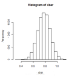
## the mean estimate is 0.7781 the sample standard deviation is 0.1016

對于Moving block bootstrap，我們有：

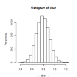
## the mean estimate is 0.7896 the sample standard deviation is 0.1114

在tseries包中提供了tsbootstrap函數，來完成block Bootstrap過程。函數調用格式如下：

tsbootstrap(x, nb = 1, statistic = NULL, m = 1, b = NULL, type = c(“stationary”,“block”), …)

參數說明：

x:原始數據，必須是數值向量或時序列

nb:Bootstrap數據集個數

statistic：Bootstrap統計量

我們可以將上面的例子利用tsbootstrap函數再算一次：

data <- read.table("D:/R/data/dgnp82.txt")
    gnp <- data * 100
    gnp1 <- ts(gnp, fre = 4, start = c(1947, 2))
    tsbootstrap(gnp1, nb = 500, mean, type = "block")

##
## Call:
## tsbootstrap(x = gnp1, nb = 500, statistic = mean, type = "block")
##
## Resampled Statistic(s):
## original bias std. error
## 0.7741 0.0316 0.1056

這與我們算的也差不多。
　　最后，我們提一下自相關系數的Bootstrap估計，這個有些類似多元統計中用到的拉直變換的逆變換，我們僅通過tsbootstrap提供的example來看看，具體內容可以參閱Paolo Giudici et al.的*Computational Statistic*一書。

n <- 500 # Generate AR(1) process
    a <- 0.6
    e <- rnorm(n + 100)
    x <- double(n + 100)
    x[1] <- rnorm(1)
    for (i in 2:(n + 100)) {
        x[i] <- a * x[i - 1] + e[i]
    }
    x <- ts(x[-(1:100)])

    acflag1 <- function(x) {
        xo <- c(x[, 1], x[1, 2])
        xm <- mean(xo)
        return(mean((x[, 1] - xm) * (x[, 2] - xm))/mean((xo - xm)^2))
    }

    tsbootstrap(x, nb = 500, statistic = acflag1, m = 2)

##
## Call:
## tsbootstrap(x = x, nb = 500, statistic = acflag1, m = 2)
##
## Resampled Statistic(s):
## original bias std. error
## 0.61538 -0.00549 0.02701

Bootstrap置信區間

說到Bootstrap推斷總會說到假設檢驗與置信區間。那么Bootstrap的置信區間如何求解呢？
一般來說有以下幾種方法：

標準正態Bootstrap置信區間

基本Bootstrap置信區間

分位數Bootstrap置信區間

Bootstrap t置信區間

BCa 置信區間

先說說標準正態Bootstrap置信區間，這是通過構造偽Z統計量($ z=\frac{\hat{\theta}-E(\hat{\theta})}{se(\hat{\theta})} $)，假設Z服從正態分布，根據Z的分位數來構造置信區間，當然假設Z服從t分布也是可以的。

基本的Bootstrap置信區間是由置信區間的定義\[ P ( L < \hat{\theta}-\theta < U )=1- \alpha \]得到的啟發,利用Bootstrap分位數$ \hat{\theta}_{U}^{*} $和$ \hat{\theta}_{L}^{*} $來估計統計量的置信區間，即通過\[ P(\hat{\theta}_{L}^{*}-\hat{\theta}<\theta^{*}-\hat{\theta}<\hat{\theta}_{U}^{*}-\hat{\theta})\approx1-\alpha \]可以將區間估計為：\[ (2\hat{\theta} - \hat{\theta}_{U}^{*}\hspace{1em} ,\hspace{1em} 2\hat{\theta}-\hat{\theta}_{L}^{*}) \]

分位數Bootstrap的想法比較簡單：既然我們將Bootstrap數據集求出的統計量的經驗分布視為統計量的分布，那么它的置信區間自然就應該是這個統計量的上下兩側的分位數。
　　Bootstrap t置信區間又稱為學生Bootstrap置信區間，它是通過Bootstrap構造偽t統計量($ t=\frac{\hat{\theta}-E(\hat{\theta})}{se(\hat{\theta})} $)，這與正態Bootstrap置信區間類似，但是這與正態Bootstrap不同的是，統計量t并不是簡單的服從student-t分布，而是構造Bootstrap數據集時，利用這個Bootstrap數據集再次進行Bootstrap，得到一個t統計量，由于我們有m個Bootstrap數據集，那么我們就有m個t統計量，利用這些t統計量的分位數作為t分布的分位數，求取置信區間。這里我們嵌套了一個Bootstrap是為了求出偽t統計量的方差，這在一些文獻中又被稱為經驗Bootstrap t置信區間。我們有時也會利用delta method 求解t統計量的方差，它的好處就在于不需要通過額外的Bootstrap求解方差了，時間上有優化，但是精度方面，究竟誰最優，還是有待商榷的。
　　BCa區間的想法是：分位數Bootstrap置信區間可能由于偏差或者偏度使得估計量沒有那么好的覆蓋率，我們聲稱的置信水平$ \alpha $可能并不對應$ \alpha $分位數，那么我就對估計量施加一個變換，使得它的偏差與偏度得到修正，那么就找到$ \alpha $實際對應的分位數，利用實際的分位數給出估計。這是由Efron于1987年提出的，如果偏差與偏度都是0的話，它就是分位數法求出的置信區間了。偏差的修正是利用中位數的偏差來進行修正，偏度的修正是利用Jackknife估計得到的。
　　boot包里的boot.ci函數可以輕松地計算這5種置信區間，其調用格式為：

boot.ci(boot.out, conf = 0.95, type = “all”, index = 1:min(2,length(boot.out$t0)), var.t0 = NULL, var.t = NULL, t0 = NULL, t = NULL, L = NULL, h = function(t) t, hdot = function(t) rep(1,length(t)), hinv = function(t) t, …)

我們以computational statistics一書的Copper-Nickel Alloy數據為例說明這個函數的使用：

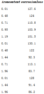
這個數據是關于金屬腐蝕與金屬體積的數據，我們要估計的估計量為以腐蝕損失為響應變量的回歸的自變量回歸系數與截距項之比，（這里我們不考慮估計量的意義），這里我們可以利用delta方法，認為估計量就是兩個回歸系數的估計量之比。

    theta.boot <- function(dat, ind) {
        y <- dat[ind, 1]
        z <- dat[ind, 2]
        theta <- as.numeric(coef(lm(z ~ y))[2]/coef(lm(z ~ y))[1])
        model <- lm(z ~ y)
        cov.m <- summary(lm(z ~ y))$cov
        theta.var <- (theta^2) * (cov.m[2, 2]/(model$coef[2]^2) + cov.m[1, 1]/(model$coef[1]^2) -
            2 * cov.m[1, 2]/(prod(model$coef)))
        theta.var <- as.numeric((theta.var))
        c(theta, theta.var)
    }
    dat <- read.table("D:/R/data/alloy.txt", head = TRUE)
    boot.obj <- boot(dat, statistic = theta.boot, R = 2000)
    print(boot.obj)
##
## ORDINARY NONPARAMETRIC BOOTSTRAP
##
##
## Call:
## boot(data = dat, statistic = theta.boot, R = 2000)
##
##
## Bootstrap Statistics :
##       original     bias    std. error
## t1* -1.851e-01 -1.270e-03   8.342e-03
## t2* 7.466e-06 1.373e-06   3.244e-06

    print(boot.ci(boot.obj))

## BOOTSTRAP CONFIDENCE INTERVAL CALCULATIONS
## Based on 2000 bootstrap replicates
##
## CALL :
## boot.ci(boot.out = boot.obj)
##
## Intervals :
## Level      Normal              Basic             Studentized
## 95%   (-0.2002, -0.1675 )   (-0.1971, -0.1649 )   (-0.1978, -0.1690 )
##
## Level     Percentile            BCa
## 95%   (-0.2053, -0.1730 )   (-0.2030, -0.1722 )
## Calculations and Intervals on Original Scale

這里的Bootstrap t利用的就是delta方法求解估計量$ \theta $的方差的，與經驗Bootstrap t有那么一點點的區別，我們這里也報告一個經驗Bootstrap t的置信區間好了：

boot.t.ci <- function(x, B = 500, R = 100, level = 0.95, statistic) {
        # compute the bootstrap t CI
        x <- as.matrix(x)
        n <- nrow(x)
        stat <- numeric(B)
        se <- numeric(B)
        boot.se <- function(x, R, f) {
            # local function to compute the bootstrap estimate of standard error for
            # statistic f(x)
            x <- as.matrix(x)
            m <- nrow(x)
            th <- replicate(R, expr = {
                i <- sample(1:m, size = m, replace = TRUE)
                f(x[i, ])
            })
            return(sd(th))
        }
        for (b in 1:B) {
            j <- sample(1:n, size = n, replace = TRUE)
            y <- x[j, ]
            stat[b] <- statistic(y)
            se[b] <- boot.se(y, R = R, f = statistic)
        }
        stat0 <- statistic(x)
        t.stats <- (stat - stat0)/se
        se0 <- sd(stat)
        alpha <- 1 - level
        Qt <- quantile(t.stats, c(alpha/2, 1 - alpha/2), type = 1)
        names(Qt) <- rev(names(Qt))
        CI <- rev(stat0 - Qt * se0)
    }
    stat <- function(dat) {
        z <- dat[, 2]
        y <- dat[, 1]
        theta <- as.numeric(coef(lm(z ~ y))[2]/coef(lm(z ~ y))[1])
    }
    ci <- boot.t.ci(dat, statistic = stat, B = 200, R = 50)
    print(ci)

## 2.5% 97.5% ## -0.2030 -0.1688

這個程序運行十分緩慢，我們看看他的運行時間：

system.time(boot.t.ci(dat, statistic = stat, B = 200, R = 50))

## user system elapsed## 34.46 0.04 35.32

這對于我的落后的電腦來說是個很大的打擊，估計要是不是R而是C++，matlab的話，可能會死掉吧。所以可以用delta method求解近似的估計問題，還是謹慎的使用經驗Bootstrap t吧。還有這里都是使用paired Bootstrap給出的估計，你可以用殘差法試試，看看估計區間會不會更大些。

Jackknife after bootstrap

我們前面介紹了利用Bootstrap估計給出偏差與方差的估計，而這些Bootstrap本身又是一個估計量，我們也想知道這個估計量的好壞，那么它們的偏差，方差怎么估計呢？再用一次Bootstrap，或者用一次Jackknife是一個不錯的選擇，但是這個效率是十分低下的，我們看經驗Bootstrap就知道了，這是一個讓人很厭煩的過程，在這里我們絕對不會再一次重復這個讓人火大的操作。萬幸的是，我們有一個稍微好些的辦法來解決這個問題，這就是著名的Jackknife after Bootstrap。
　　我們將算法描述如下：　　　
　　記$ X_{i}^{*} $為一次Bootstrap抽樣，$ X_{1}^{*},\cdots,X_{B}^{*} $是樣本大小為B的Bootstrap數據集，令$ J(i) $表示不含總體樣本的元素$ x_{i} $的Bootstrap數據集，我們利用$ J(i) $作為一次Jackknife重復，這有點類似delete-K Jackknife，標準差估計量的Jackknife估計為\[ \hat{se}_{jack}(\hat{se}_{Boot}(\hat{\theta}))=\sqrt{\frac{n-1}{n}\sum_{i=1}^{n}(\hat{se}_{Boot(i)}-\overline{\hat{se}_{Boot(\cdot)}})^2}\\\hat{se}_{Boot(i)}=\sqrt{\frac{1}{B(i)}\sum_{j\in J(i)}(\hat{\theta}_{(j)}-\overline{\hat{\theta}_{(J(i))}})^2}\\\overline{\hat{\theta}_{(J(i))}}=\frac{1}{B(i)}\sum_{j\in J(i)}\hat{\theta}_{(j)} \]其中B(i)表示不含$ x_{i} $的樣本個數。
　　我們來看金屬腐蝕與金屬體積數據的估計量的方差的方差的估計：

dat <- read.table("D:/R/data/alloy.txt", head = TRUE)
    n <- nrow(dat)
    y <- dat[, 2]
    z <- dat[, 1]
    B <- 2000
    theta.b <- numeric(B)
    # set up storage for the sampled indices
    indices <- matrix(0, nrow = B, ncol = n)
    # jackknife-after-bootstrap step 1: run the bootstrap
    for (b in 1:B) {
        i <- sample(1:n, size = n, replace = TRUE)
        y <- dat[i, 2]
        z <- dat[i, 1]
        theta.b[b] <- as.numeric(coef(lm(z ~ y))[2]/coef(lm(z ~ y))[1])
        # save the indices for the jackknife
        indices[b, ] <- i
    }
    # jackknife-after-bootstrap to est. se(se)
    se.jack <- numeric(n)
    for (i in 1:n) {
        # in i-th replicate omit all samples with x[i]
        keep <- (1:B)[apply(indices, MARGIN = 1, FUN = function(k) {
            !any(k == i)
        })]
        se.jack[i] <- sd(theta.b[keep])
    }
    print(sd(theta.b))

## [1] 8.838e-05

Bootstrap的方差縮減問題

要知道方差縮減，首先需要明白方差來源于何處？對于Bootstrap而言，方差的來源主要有兩個方面：一個是原始樣本抽樣的方差，另一個是Bootstrap抽樣產生的方差。
　　原始樣本抽樣的方差在這里我們假定是沒法改進的，那么Bootstrap抽樣的方差該如何減少呢？這可以借鑒Monte Carlo中的方差縮減技術，采用重要抽樣，關聯抽樣等辦法，其中關聯抽樣的方法運用于Bootstrap，就產生了平衡Bootstrap與方向Bootstrap兩種方法。