python實現邏輯回歸的方法示例

這篇文章主要介紹了python實現邏輯回歸的方法示例，這是機器學習課程的一個實驗，整理出來共享給大家，

本文實現的原理很簡單，優化方法是用的梯度下降。后面有測試結果。

先來看看實現的示例代碼：    
# coding=utf-8
from math import exp
 
import matplotlib.pyplot as plt
import numpy as np
from sklearn.datasets.samples_generator import make_blobs
 
 
def sigmoid(num):
 '''
 
 :param num: 待計算的x
 :return: sigmoid之后的數值
 '''
 if type(num) == int or type(num) == float:
  return 1.0 / (1 + exp(-1 * num))
 else:
  raise ValueError, 'only int or float data can compute sigmoid'
 
 
class logistic():
 def __init__(self, x, y):
  if type(x) == type(y) == list:
   self.x = np.array(x)
   self.y = np.array(y)
  elif type(x) == type(y) == np.ndarray:
   self.x = x
   self.y = y
  else:
   raise ValueError, 'input data error'
 
 def sigmoid(self, x):
  '''
 
  :param x: 輸入向量
  :return: 對輸入向量整體進行simgoid計算后的向量結果
  '''
  s = np.frompyfunc(lambda x: sigmoid(x), 1, 1)
  return s(x)
 
 def train_with_punish(self, alpha, errors, punish=0.0001):
  '''
 
  :param alpha: alpha為學習速率
  :param errors: 誤差小于多少時停止迭代的閾值
  :param punish: 懲罰系數
  :param times: 最大迭代次數
  :return:
  '''
  self.punish = punish
  dimension = self.x.shape[1]
  self.theta = np.random.random(dimension)
  compute_error = 100000000
  times = 0
  while compute_error > errors:
   res = np.dot(self.x, self.theta)
   delta = self.sigmoid(res) - self.y
   self.theta = self.theta - alpha * np.dot(self.x.T, delta) - punish * self.theta # 帶懲罰的梯度下降方法
   compute_error = np.sum(delta)
   times += 1
 
 def predict(self, x):
  '''
 
  :param x: 給入新的未標注的向量
  :return: 按照計算出的參數返回判定的類別
  '''
  x = np.array(x)
  if self.sigmoid(np.dot(x, self.theta)) > 0.5:
   return 1
  else:
   return 0
 
 
def test1():
 '''
 用來進行測試和畫圖，展現效果
 :return:
 '''
 x, y = make_blobs(n_samples=200, centers=2, n_features=2, random_state=0, center_box=(10, 20))
 x1 = []
 y1 = []
 x2 = []
 y2 = []
 for i in range(len(y)):
  if y[i] == 0:
   x1.append(x[i][0])
   y1.append(x[i][1])
  elif y[i] == 1:
   x2.append(x[i][0])
   y2.append(x[i][1])
 # 以上均為處理數據，生成出兩類數據
 p = logistic(x, y)
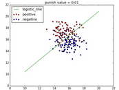
 p.train_with_punish(alpha=0.00001, errors=0.005, punish=0.01) # 步長是0.00001，最大允許誤差是0.005，懲罰系數是0.01
 x_test = np.arange(10, 20, 0.01)
 y_test = (-1 * p.theta[0] / p.theta[1]) * x_test
 plt.plot(x_test, y_test, c='g', label='logistic_line')
 plt.scatter(x1, y1, c='r', label='positive')
 plt.scatter(x2, y2, c='b', label='negative')
 plt.legend(loc=2)
 plt.title('punish value = ' + p.punish.__str__())
 plt.show()
 
 
if __name__ == '__main__':
 test1()

運行結果如下圖

總結
以上就是這篇文章的全部內容了，希望本文的內容對大家的學習或者工作能帶來一定的幫助