R做線性回歸及檢驗

使用R對內置鳶尾花數據集iris（在R提示符下輸入iris回車可看到內容）進行回歸分析，自行選擇因變量和自變量，注意Species這個分類變量的處理方法

## 將iris數據加載進來
attach(iris)
## 查看iris數據的整體情況
str(iris)
## 'data.frame':    150 obs. of  5 variables:
##  $ Sepal.Length: num  5.1 4.9 4.7 4.6 5 5.4 4.6 5 4.4 4.9 ...
##  $ Sepal.Width : num  3.5 3 3.2 3.1 3.6 3.9 3.4 3.4 2.9 3.1 ...
##  $ Petal.Length: num  1.4 1.4 1.3 1.5 1.4 1.7 1.4 1.5 1.4 1.5 ...
##  $ Petal.Width : num  0.2 0.2 0.2 0.2 0.2 0.4 0.3 0.2 0.2 0.1 ...
##  $ Species     : Factor w/ 3 levels "setosa","versicolor",..: 1 1 1 1 1 1 1 1 1 1 ...
可以看出，共有150個樣本，5個變量，前四個是數值型，第五個變量是因子型。
## 查看數據散點分布情況
pairs(iris[, 1:4], col = "blue")

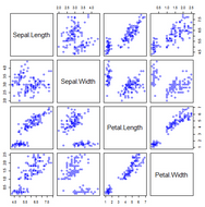
從上圖可以看出，Sepal.Length與Petal.Length、Petal.Length與Petal.Width存在明顯的正相關性。接下來選擇這兩對變量分別建立回歸模型。

(lm1 <- lm(Sepal.Length ~ Petal.Length))
## 
## Call:
## lm(formula = Sepal.Length ~ Petal.Length)
## 
## Coefficients:
##  (Intercept)  Petal.Length  
##        4.307         0.409
(lm2 <- lm(Petal.Length ~ Petal.Width))
## 
## Call:
## lm(formula = Petal.Length ~ Petal.Width)
## 
## Coefficients:
## (Intercept)  Petal.Width  
##        1.08         2.23
summary(lm1)
## 
## Call:
## lm(formula = Sepal.Length ~ Petal.Length)
## 
## Residuals:
##     Min      1Q  Median      3Q     Max 
## -1.2468 -0.2966 -0.0152  0.2768  1.0027 
## 
## Coefficients:
##              Estimate Std. Error t value Pr(>|t|)    
## (Intercept)    4.3066     0.0784    54.9   <2e-16 ***
## Petal.Length   0.4089     0.0189    21.6   <2e-16 ***
## ---
## Signif. codes:  0 '***' 0.001 '**' 0.01 '*' 0.05 '.' 0.1 ' ' 1
## 
## Residual standard error: 0.407 on 148 degrees of freedom
## Multiple R-squared:  0.76,   Adjusted R-squared:  0.758 
## F-statistic:  469 on 1 and 148 DF,  p-value: <2e-16
summary(lm2)
## 
## Call:
## lm(formula = Petal.Length ~ Petal.Width)
## 
## Residuals:
##     Min      1Q  Median      3Q     Max 
## -1.3354 -0.3035 -0.0295  0.2578  1.3945 
## 
## Coefficients:
##             Estimate Std. Error t value Pr(>|t|)    
## (Intercept)   1.0836     0.0730    14.8   <2e-16 ***
## Petal.Width   2.2299     0.0514    43.4   <2e-16 ***
## ---
## Signif. codes:  0 '***' 0.001 '**' 0.01 '*' 0.05 '.' 0.1 ' ' 1
## 
## Residual standard error: 0.478 on 148 degrees of freedom
## Multiple R-squared:  0.927,  Adjusted R-squared:  0.927 
## F-statistic: 1.88e+03 on 1 and 148 DF,  p-value: <2e-16
兩個模型的擬合效果都不錯，但從R平方和角度考慮，lm2的模型效果好點。
##對建立的模型分別進行殘差檢驗
par(mfrow = c(2, 2))
plot(lm1)

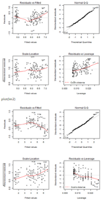
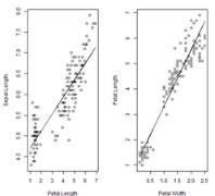
par(mfrow = c(1, 2))
plot(Petal.Length, Sepal.Length)
lines(Petal.Length, lm1$fitted.values)
plot(Petal.Width, Petal.Length)
lines(Petal.Width, lm2$fitted.values)

數據中的第五個變量Species是因子型變量，在進行回歸建模前，需要對其進行啞變量處理，提高模型精確度。在R建立回歸模型時，會主動對因子型變量進行啞變量處理，下面先利用Sepal.Width、Species對Sepal.Length建立回歸模型，看看效果。

lm3 <- lm(Sepal.Length ~ Sepal.Width + Species)
summary(lm3)
## 
## Call:
## lm(formula = Sepal.Length ~ Sepal.Width + Species)
## 
## Residuals:
##     Min      1Q  Median      3Q     Max 
## -1.3071 -0.2571 -0.0533  0.1954  1.4125 
## 
## Coefficients:
##                   Estimate Std. Error t value Pr(>|t|)    
## (Intercept)          2.251      0.370    6.09  9.6e-09 ***
## Sepal.Width          0.804      0.106    7.56  4.2e-12 ***
## Speciesversicolor    1.459      0.112   13.01  < 2e-16 ***
## Speciesvirginica     1.947      0.100   19.47  < 2e-16 ***
## ---
## Signif. codes:  0 '***' 0.001 '**' 0.01 '*' 0.05 '.' 0.1 ' ' 1
## 
## Residual standard error: 0.438 on 146 degrees of freedom
## Multiple R-squared:  0.726,  Adjusted R-squared:  0.72 
## F-statistic:  129 on 3 and 146 DF,  p-value: <2e-16
par(mfrow = c(2, 2))
plot(lm3)

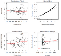
從建立的模型的各系數的p值看出，各參量均是顯著的。R平方和也有0.726，處于一個相對合理的水平。故該模型是可以接受的。

2 使用R對內置longley數據集進行回歸分析，如果以GNP.deflator作為因變量y，問這個數據集是否存在多重共線性問題？應該選擇哪些變量參與回歸？

答：

## 查看longley的數據結構
str(longley)
## 'data.frame':    16 obs. of  7 variables:
##  $ GNP.deflator: num  83 88.5 88.2 89.5 96.2 ...
##  $ GNP         : num  234 259 258 285 329 ...
##  $ Unemployed  : num  236 232 368 335 210 ...
##  $ Armed.Forces: num  159 146 162 165 310 ...
##  $ Population  : num  108 109 110 111 112 ...
##  $ Year        : int  1947 1948 1949 1950 1951 1952 1953 1954 1955 1956 ...
##  $ Employed    : num  60.3 61.1 60.2 61.2 63.2 ...
longly數據集中有7個變量16個觀測值，7個變量均屬于數值型。

首先建立全量回歸模型
lm1 <- lm(GNP.deflator ~ ., data = longley)
summary(lm1)
## 
## Call:
## lm(formula = GNP.deflator ~ ., data = longley)
## 
## Residuals:
##    Min     1Q Median     3Q    Max 
## -2.009 -0.515  0.113  0.423  1.550 
## 
## Coefficients:
##               Estimate Std. Error t value Pr(>|t|)  
## (Intercept)  2946.8564  5647.9766    0.52    0.614  
## GNP             0.2635     0.1082    2.44    0.038 *
## Unemployed      0.0365     0.0302    1.21    0.258  
## Armed.Forces    0.0112     0.0155    0.72    0.488  
## Population     -1.7370     0.6738   -2.58    0.030 *
## Year           -1.4188     2.9446   -0.48    0.641  
## Employed        0.2313     1.3039    0.18    0.863  
## ---
## Signif. codes:  0 '***' 0.001 '**' 0.01 '*' 0.05 '.' 0.1 ' ' 1
## 
## Residual standard error: 1.19 on 9 degrees of freedom
## Multiple R-squared:  0.993,  Adjusted R-squared:  0.988 
## F-statistic:  203 on 6 and 9 DF,  p-value: 4.43e-09
建立的模型結果是令人沮喪的，6個變量的顯著性p值只有兩個有一顆星，說明有些變量不適合用于建模。

看各自變量是否存在共線性問題。此處利用方差膨脹因子進行判斷：方差膨脹因子VIF是指回歸系數的估計量由于自變量共線性使得方差增加的一個相對度量。一般建議，如VIF>10，表明模型中有很強的共線性問題。
library(car)
vif(lm1, digits = 3)
##          GNP   Unemployed Armed.Forces   Population         Year 
##      1214.57        83.96        12.16       230.91      2065.73 
##     Employed 
##       220.42
從結果看，所有自變量的vif值均超過了10，其中GNP、Year更是高達四位數，存在嚴重的多種共線性。接下來，利用cor（）函數查看各自變量間的相關系數。
plot(longley[, 2:7])

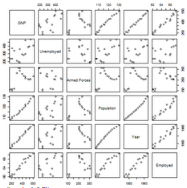
cor(longley[, 2:7])
##                 GNP Unemployed Armed.Forces Population   Year Employed
## GNP          1.0000     0.6043       0.4464     0.9911 0.9953   0.9836
## Unemployed   0.6043     1.0000      -0.1774     0.6866 0.6683   0.5025
## Armed.Forces 0.4464    -0.1774       1.0000     0.3644 0.4172   0.4573
## Population   0.9911     0.6866       0.3644     1.0000 0.9940   0.9604
## Year         0.9953     0.6683       0.4172     0.9940 1.0000   0.9713
## Employed     0.9836     0.5025       0.4573     0.9604 0.9713   1.0000
從散點分布圖和相關系數，均可以得知，自變量間存在嚴重共線性。
接下來利用step（）函數進行變量的初步篩選。
lm1.step <- step(lm1, direction = "backward")
## Start:  AIC=10.48
## GNP.deflator ~ GNP + Unemployed + Armed.Forces + Population + 
##     Year + Employed
## 
##                Df Sum of Sq  RSS   AIC
## - Employed      1      0.04 12.9  8.54
## - Year          1      0.33 13.2  8.89
## - Armed.Forces  1      0.74 13.6  9.39
##                     12.8 10.48
## - Unemployed    1      2.08 14.9 10.88
## - GNP           1      8.47 21.3 16.59
## - Population    1      9.48 22.3 17.33
## 
## Step:  AIC=8.54
## GNP.deflator ~ GNP + Unemployed + Armed.Forces + Population + 
##     Year
## 
##                Df Sum of Sq  RSS   AIC
## - Year          1      0.46 13.3  7.11
##                     12.9  8.54
## - Armed.Forces  1      1.79 14.7  8.62
## - Unemployed    1      5.74 18.6 12.43
## - GNP           1      9.40 22.3 15.30
## - Population    1      9.90 22.8 15.66
## 
## Step:  AIC=7.11
## GNP.deflator ~ GNP + Unemployed + Armed.Forces + Population
## 
##                Df Sum of Sq  RSS   AIC
## - Armed.Forces  1       1.3 14.7  6.62
##                     13.4  7.11
## - Population    1       9.7 23.0 13.82
## - Unemployed    1      14.5 27.8 16.86
## - GNP           1      35.2 48.6 25.76
## 
## Step:  AIC=6.62
## GNP.deflator ~ GNP + Unemployed + Population
## 
##              Df Sum of Sq  RSS   AIC
##                   14.7  6.62
## - Unemployed  1      13.3 28.0 14.95
## - Population  1      13.3 28.0 14.95
## - GNP         1      48.6 63.2 27.99
根據AIC 赤池信息準則，模型最后選擇Unemployed、Population、GNP三個因變量參與建模。
查看進行逐步回歸后的模型效果
summary(lm1.step)
## 
## Call:
## lm(formula = GNP.deflator ~ GNP + Unemployed + Population, data = longley)
## 
## Residuals:
##    Min     1Q Median     3Q    Max 
## -2.047 -0.682  0.196  0.696  1.435 
## 
## Coefficients:
##              Estimate Std. Error t value Pr(>|t|)    
## (Intercept) 221.12959   48.97251    4.52  0.00071 ***
## GNP           0.22010    0.03493    6.30  3.9e-05 ***
## Unemployed    0.02246    0.00681    3.30  0.00634 ** 
## Population   -1.80501    0.54692   -3.30  0.00634 ** 
## ---
## Signif. codes:  0 '***' 0.001 '**' 0.01 '*' 0.05 '.' 0.1 ' ' 1
## 
## Residual standard error: 1.11 on 12 degrees of freedom
## Multiple R-squared:  0.992,  Adjusted R-squared:  0.989 
## F-statistic:  472 on 3 and 12 DF,  p-value: 1.03e-12
從各判定指標可以看出，模型的結果是可喜的。參與建模的三個變量和截距均是顯著的。R平方和也高達0.992。