數據可視化發現「吃雞」秘密

大吉大利，今晚吃雞~

今天跟朋友玩了幾把吃雞，經歷了各種死法，還被嘲笑說論女生吃雞的100種死法，比如被拳頭掄死、跳傘落到房頂邊緣摔死 、把吃雞玩成飛車被車技秀死、被隊友用燃燒瓶燒死的。這種游戲對我來說就是一個讓我明白原來還有這種死法的游戲。

但是玩歸玩，還是得假裝一下我沉迷學習，所以今天就用吃雞比賽的真實數據來看看，如何提高你吃雞的概率。

那么我們就用Python和R做數據分析來回答以下的靈魂發問。

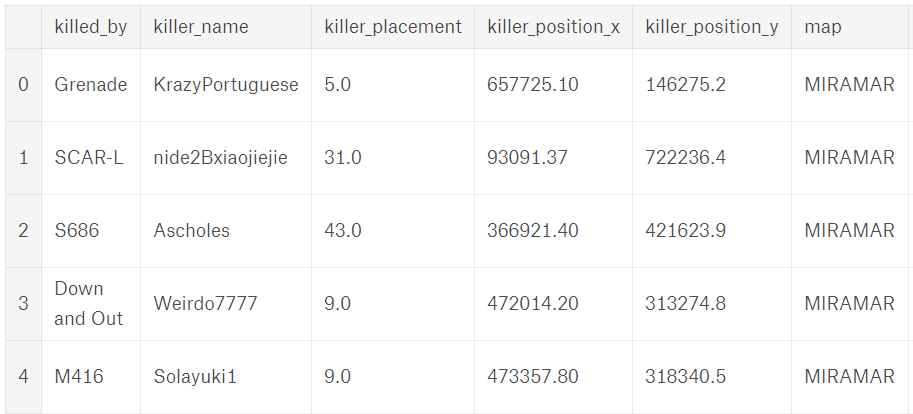
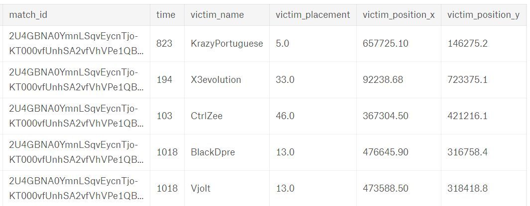
首先來看下數據：

1、跳哪兒危險？

對于我這樣一直喜歡茍著的良心玩家，在經歷了無數次落地成河的慘痛經歷后，我是堅決不會選擇跳P城這樣樓房密集的城市，窮歸窮但保命要緊。

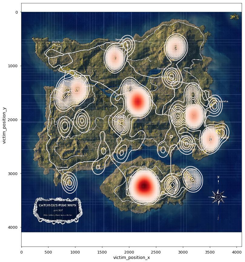
所以我們決定統計一下，到底哪些地方更容易落地成河？

我們篩選出在前100秒死亡的玩家地點進行可視化分析。激情沙漠地圖的電站、皮卡多、別墅區、依波城最為危險，火車站、火電廠相對安全。絕地海島中P城、軍事基地、學校、醫院、核電站、防空洞都是絕對的危險地帶。物質豐富的G港居然相對安全。

1importnumpyasnp

2importmatplotlib.pyplotasplt

3importpandasaspd

4importseabornassns

5fromscipy.misc.pilutilimportimread

6importmatplotlib.cmascm

7

8#導入部分數據

9deaths1 = pd.read_csv("deaths/kill_match_stats_final_0.csv")

10deaths2 = pd.read_csv("deaths/kill_match_stats_final_1.csv")

11

12deaths = pd.concat([deaths1, deaths2])

13

14#打印前5列，理解變量

15print(deaths.head(),'n',len(deaths))

16

17#兩種地圖

18miramar = deaths[deaths["map"] =="MIRAMAR"]

19erangel = deaths[deaths["map"] =="ERANGEL"]

20

21#開局前100秒死亡熱力圖

22position_data = ["killer_position_x","killer_position_y","victim_position_x","victim_position_y"]

23forpositioninposition_data:

24miramar[position] = miramar[position].apply(lambdax: x*1000/800000)

25miramar = miramar[miramar[position] !=0]

26

27erangel[position] = erangel[position].apply(lambdax: x*4096/800000)

28erangel = erangel[erangel[position] !=0]

29

30n =50000

31mira_sample = miramar[miramar["time"] <100].sample(n)

32eran_sample = erangel[erangel["time"] <100].sample(n)

33

34# miramar熱力圖

35bg = imread("miramar.jpg")

36fig, ax = plt.subplots(1,1,figsize=(15,15))

37ax.imshow(bg)

38sns.kdeplot(mira_sample["victim_position_x"], mira_sample["victim_position_y"],n_levels=100, cmap=cm.Reds, alpha=0.9)

39

40# erangel熱力圖

41bg = imread("erangel.jpg")

42fig, ax = plt.subplots(1,1,figsize=(15,15))

43ax.imshow(bg)

44sns.kdeplot(eran_sample["victim_position_x"], eran_sample["victim_position_y"], n_levels=100,cmap=cm.Reds, alpha=0.9)

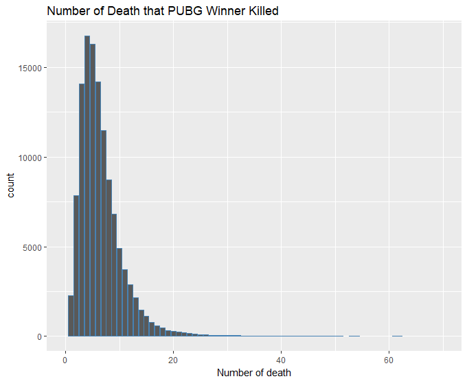
2、茍著還是出去干？

我到底是茍在房間里面還是出去和敵人硬拼？

這里因為比賽的規模不一樣，這里選取參賽人數大于90的比賽數據，然后篩選出團隊team_placement即最后成功吃雞的團隊數據。

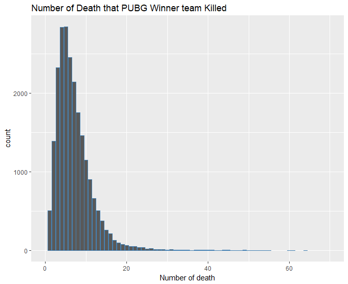
1、先計算了吃雞團隊平均擊殺敵人的數量，這里剔除了四人模式的比賽數據，因為人數太多的團隊會因為數量懸殊平均而變得沒意義；

2、所以我們考慮通過分組統計每一組吃雞中存活到最后的成員擊殺敵人的數量，但是這里發現數據統計存活時間變量是按照團隊最終存活時間記錄的，所以該想法失??；

3、最后統計每個吃雞團隊中擊殺人數最多的數量統計，這里剔除了單人模式的數據，因為單人模式的數量就是每組擊殺最多的數量。

最后居然發現還有擊殺數量達到60的，懷疑是否有開掛。想要吃雞還是得出去練槍法，光是茍著是不行的。

1library(dplyr)

2library(tidyverse)

3library(data.table)

4library(ggplot2)

5pubg_full <- fread("../agg_match_stats.csv")

6# 吃雞團隊平均擊殺敵人的數量

7attach(pubg_full)

8pubg_winner <- pubg_full %>% filter(team_placement==1&party_size<4&game_size>90)

9detach(pubg_full)

10team_killed <- aggregate(pubg_winner$player_kills, by=list(pubg_winner$match_id,pubg_winner$team_id), FUN="mean")

11team_killed$death_num <- ceiling(team_killed$x)

12ggplot(data = team_killed) + geom_bar(mapping = aes(x = death_num, y = ..count..), color="steelblue") +

13xlim(0,70) + labs(title ="Number of Death that PUBG Winner team Killed", x="Number of death")

14

15# 吃雞團隊最后存活的玩家擊殺數量

16pubg_winner <- pubg_full %>% filter(pubg_full$team_placement==1) %>% group_by(match_id,team_id)

17attach(pubg_winner)

18team_leader <- aggregate(player_survive_time~player_kills, data = pubg_winner, FUN="max")

19detach(pubg_winner)

20

21# 吃雞團隊中擊殺敵人最多的數量

22pubg_winner <- pubg_full %>% filter(pubg_full$team_placement==1&pubg_full$party_size>1)

23attach(pubg_winner)

24team_leader <- aggregate(player_kills, by=list(match_id,team_id), FUN="max")

25detach(pubg_winner)

26ggplot(data = team_leader) + geom_bar(mapping = aes(x = x, y = ..count..), color="steelblue") +

27xlim(0,70) + labs(title ="Number of Death that PUBG Winner Killed", x="Number of death")

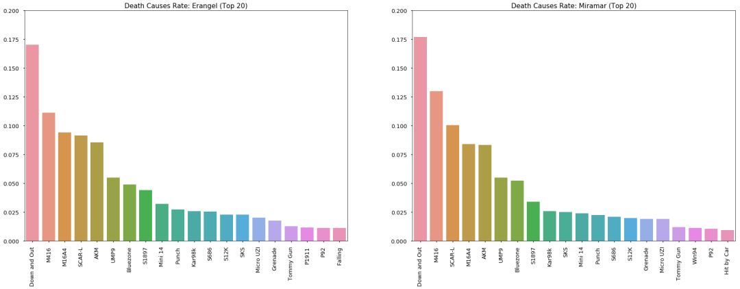
3、哪一種武器干掉的玩家多？

運氣好挑到好武器的時候，你是否猶豫選擇哪一件？

從圖上來看，M416和SCAR是不錯的武器，也是相對容易能撿到的武器，大家公認Kar98k是能一槍斃命的好槍，它排名比較靠后的原因也是因為這把槍在比賽比較難得，而且一下擊中敵人也是需要實力的，像我這種撿到98k還裝上8倍鏡但沒捂熱乎1分鐘的玩家是不配得到它的。（捂臉）

1#殺人武器排名

2death_causes = deaths['killed_by'].value_counts()

3

4sns.set_context('talk')

5fig = plt.figure(figsize=(30,10))

6ax = sns.barplot(x=death_causes.index, y=[v / sum(death_causes)forvindeath_causes.values])

7ax.set_title('Rate of Death Causes')

8ax.set_xticklabels(death_causes.index, rotation=90)

9

10#排名前20的武器

11rank =20

12fig = plt.figure(figsize=(20,10))

13ax = sns.barplot(x=death_causes[:rank].index, y=[v / sum(death_causes)forvindeath_causes[:rank].values])

14ax.set_title('Rate of Death Causes')

15ax.set_xticklabels(death_causes.index, rotation=90)

16

17#兩個地圖分開取

18f, axes = plt.subplots(1,2, figsize=(30,10))

19axes[0].set_title('Death Causes Rate: Erangel (Top {})'.format(rank))

20axes[1].set_title('Death Causes Rate: Miramar (Top {})'.format(rank))

21

22counts_er = erangel['killed_by'].value_counts()

23counts_mr = miramar['killed_by'].value_counts()

24

25sns.barplot(x=counts_er[:rank].index, y=[v / sum(counts_er)forvincounts_er.values][:rank], ax=axes[0] )

26sns.barplot(x=counts_mr[:rank].index, y=[v / sum(counts_mr)forvincounts_mr.values][:rank], ax=axes[1] )

27axes[0].set_ylim((0,0.20))

28axes[0].set_xticklabels(counts_er.index, rotation=90)

29axes[1].set_ylim((0,0.20))

30axes[1].set_xticklabels(counts_mr.index, rotation=90)

31

32#吃雞和武器的關系

33win = deaths[deaths["killer_placement"] ==1.0]

34win_causes = win['killed_by'].value_counts()

35

36sns.set_context('talk')

37fig = plt.figure(figsize=(20,10))

38ax = sns.barplot(x=win_causes[:20].index, y=[v / sum(win_causes)forvinwin_causes[:20].values])

39ax.set_title('Rate of Death Causes of Win')

40ax.set_xticklabels(win_causes.index, rotation=90)

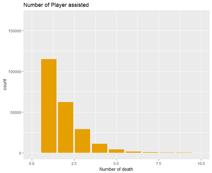
4、隊友的助攻是否助我吃雞？

有時候一不留神就被擊倒了，還好我爬得快讓隊友救我。這里選擇成功吃雞的隊伍，最終接受1次幫助的成員所在的團隊吃雞的概率為29%，所以說隊友助攻還是很重要的（再不要罵我豬隊友了，我也可以選擇不救你）。竟然還有讓隊友救9次的，你也是個人才。（手動滑稽)

1library(dplyr)

2library(tidyverse)

3library(data.table)

4library(ggplot2)

5pubg_full <- fread("E:/aggregate/agg_match_stats_0.csv")

6attach(pubg_full)

7pubg_winner <- pubg_full %>% filter(team_placement==1)

8detach(pubg_full)

9ggplot(data = pubg_winner) + geom_bar(mapping = aes(x = player_assists, y = ..count..), fill="#E69F00") +

10xlim(0,10) + labs(title ="Number of Player assisted", x="Number of death")

11ggplot(data = pubg_winner) + geom_bar(mapping = aes(x = player_assists, y = ..prop..), fill="#56B4E9") +

12xlim(0,10) + labs(title ="Number of Player assisted", x="Number of death")

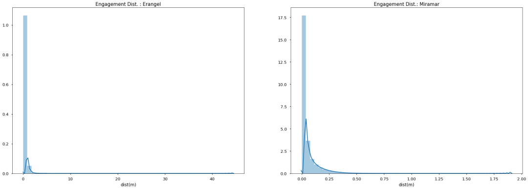
5、敵人離我越近越危險？

對數據中的killer_position和victim_position變量進行歐式距離計算，查看兩者的直線距離跟被擊倒的分布情況，呈現一個明顯的右偏分布，看來還是需要隨時觀察到附近的敵情，以免到淘汰都不知道敵人在哪兒。

1# python代碼：殺人和距離的關系

2importmath

3defget_dist(df):#距離函數

4dist = []

5forrowindf.itertuples():

6subset = (row.killer_position_x - row.victim_position_x)**2+ (row.killer_position_y - row.victim_position_y)**2

7ifsubset >0:

8dist.append(math.sqrt(subset) /100)

9else:

10dist.append(0)

11returndist

12

13df_dist = pd.DataFrame.from_dict({'dist(m)': get_dist(erangel)})

14df_dist.index = erangel.index

15

16erangel_dist = pd.concat([erangel,df_dist], axis=1)

17

18df_dist = pd.DataFrame.from_dict({'dist(m)': get_dist(miramar)})

19df_dist.index = miramar.index

20

21miramar_dist = pd.concat([miramar,df_dist], axis=1)

22

23f, axes = plt.subplots(1,2, figsize=(30,10))

24plot_dist =150

25

26axes[0].set_title('Engagement Dist. : Erangel')

27axes[1].set_title('Engagement Dist.: Miramar')

28

29plot_dist_er = erangel_dist[erangel_dist['dist(m)'] <= plot_dist]

30plot_dist_mr = miramar_dist[miramar_dist['dist(m)'] <= plot_dist]

31

32sns.distplot(plot_dist_er['dist(m)'], ax=axes[0])

33sns.distplot(plot_dist_mr['dist(m)'], ax=axes[1])

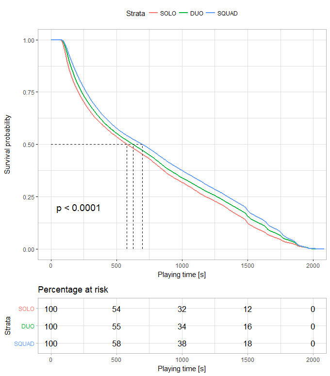
6、團隊人越多我活得越久？

對數據中的party_size變量進行生存分析，可以看到在同一生存率下，四人團隊的生存時間高于兩人團隊，再是單人模式，所以人多力量大這句話不是沒有道理的。

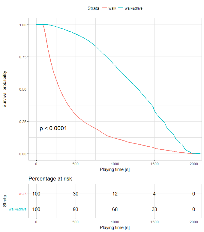
7、乘車是否活得更久？

對死因分析中發現，也有不少玩家死于Bluezone，大家天真的以為撿繃帶就能跑毒。對數據中的player_dist_ride變量進行生存分析，可以看到在同一生存率下，有開車經歷的玩家生存時間高于只走路的玩家，光靠腿你是跑不過毒的。

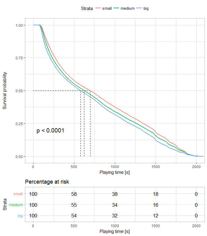
8、小島上人越多我活得更久？

對game_size變量進行生存分析發現還是小規模的比賽比較容易存活。

1# R語言代碼如下：

2library(magrittr)

3library(dplyr)

4library(survival)

5library(tidyverse)

6library(data.table)

7library(ggplot2)

8library(survminer)

9pubg_full <- fread("../agg_match_stats.csv")

10# 數據預處理，將連續變量劃為分類變量

11pubg_sub <- pubg_full %>%

12filter(player_survive_time<2100) %>%

13mutate(drive = ifelse(player_dist_ride>0,1,0)) %>%

14mutate(size = ifelse(game_size<33,1,ifelse(game_size>=33&game_size<66,2,3)))

15# 創建生存對象

16surv_object <- Surv(time = pubg_sub$player_survive_time)

17fit1 <- survfit(surv_object~party_size,data = pubg_sub)

18# 可視化生存率

19ggsurvplot(fit1, data = pubg_sub, pval =TRUE, xlab="Playing time [s]", surv.median.line="hv",

20legend.labs=c("SOLO","DUO","SQUAD"), ggtheme = theme_light(),risk.table="percentage")

21fit2 <- survfit(surv_object~drive,data=pubg_sub)

22ggsurvplot(fit2, data = pubg_sub, pval =TRUE, xlab="Playing time [s]", surv.median.line="hv",

23legend.labs=c("walk","walk&drive"), ggtheme = theme_light(),risk.table="percentage")

24fit3 <- survfit(surv_object~size,data=pubg_sub)

25ggsurvplot(fit3, data = pubg_sub, pval =TRUE, xlab="Playing time [s]", surv.median.line="hv",

26legend.labs=c("small","medium","big"), ggtheme = theme_light(),risk.table="percentage")

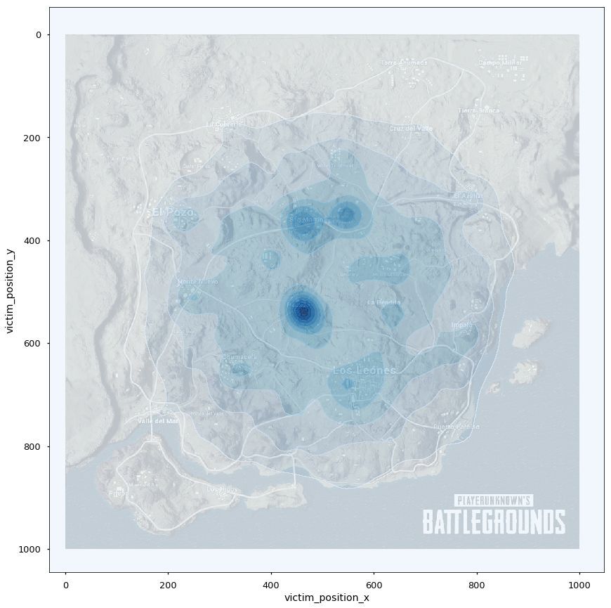
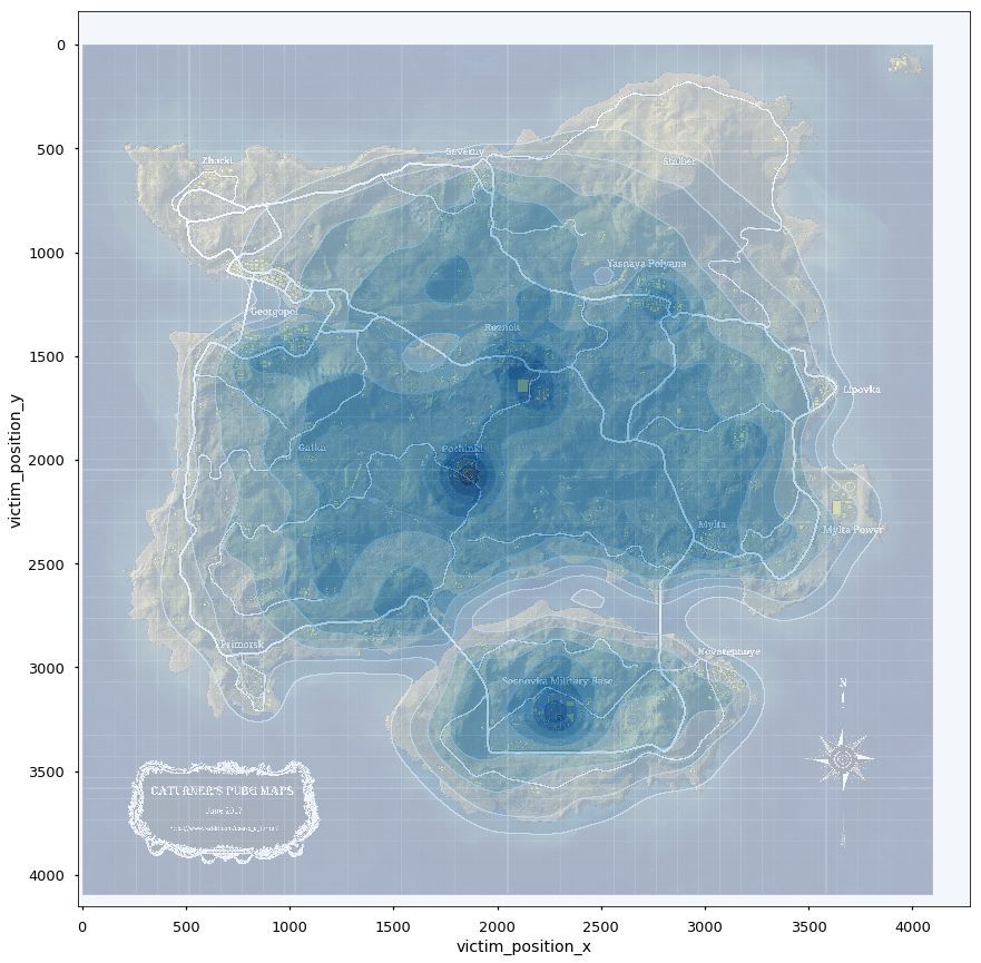
9、最后毒圈有可能出現的地點？

面對有本事能茍到最后的我，怎么樣預測最后的毒圈出現在什么位置。

從表agg_match_stats數據找出排名第一的隊伍，然后按照match_id分組，找出分組數據里面player_survive_time最大的值，然后據此匹配表格kill_match_stats_final里面的數據，這些數據里面取第二名死亡的位置，作圖發現激情沙漠的毒圈明顯更集中一些，大概率出現在皮卡多、圣馬丁和別墅區。絕地海島的就比較隨機了，但是還是能看出軍事基地和山脈的地方更有可能是最后的毒圈。

1#最后毒圈位置

2import matplotlib.pyplot as plt

3import pandas as pd

4import seaborn as sns

5from scipy.misc.pilutil import imread

6import matplotlib.cm as cm

7

8#導入部分數據

9deaths = pd.read_csv("deaths/kill_match_stats_final_0.csv")

10#導入aggregate數據

11aggregate = pd.read_csv("aggregate/agg_match_stats_0.csv")

12print(aggregate.head())

13#找出最后三人死亡的位置

14

15team_win = aggregate[aggregate["team_placement"]==1]#排名第一的隊伍

16#找出每次比賽第一名隊伍活的最久的那個player

17grouped = team_win.groupby('match_id').apply(lambda t: t[t.player_survive_time==t.player_survive_time.max()])

18

19deaths_solo = deaths[deaths['match_id'].isin(grouped['match_id'].values)]

20deaths_solo_er = deaths_solo[deaths_solo['map'] =='ERANGEL']

21deaths_solo_mr = deaths_solo[deaths_solo['map'] =='MIRAMAR']

22

23df_second_er = deaths_solo_er[(deaths_solo_er['victim_placement'] ==2)].dropna()

24df_second_mr = deaths_solo_mr[(deaths_solo_mr['victim_placement'] ==2)].dropna()

25print (df_second_er)

26

27position_data = ["killer_position_x","killer_position_y","victim_position_x","victim_position_y"]

28forpositioninposition_data:

29df_second_mr[position] = df_second_mr[position].apply(lambda x: x*1000/800000)

30df_second_mr = df_second_mr[df_second_mr[position] !=0]

31

32df_second_er[position] = df_second_er[position].apply(lambda x: x*4096/800000)

33df_second_er = df_second_er[df_second_er[position] !=0]

34

35df_second_er=df_second_er

36# erangel熱力圖

37sns.set_context('talk')

38bg = imread("erangel.jpg")

39fig, ax = plt.subplots(1,1,figsize=(15,15))

40ax.imshow(bg)

41sns.kdeplot(df_second_er["victim_position_x"], df_second_er["victim_position_y"], cmap=cm.Blues, alpha=0.7,shade=True)

42

43# miramar熱力圖

44bg = imread("miramar.jpg")

45fig, ax = plt.subplots(1,1,figsize=(15,15))

46ax.imshow(bg)

47sns.kdeplot(df_second_mr["victim_position_x"], df_second_mr["victim_position_y"], cmap=cm.Blues,alpha=0.8,shade=True)

最后祝大家：