R語言線性回歸診斷

回歸診斷主要內容
(1).誤差項是否滿足獨立性，等方差性與正態
(2).選擇線性模型是否合適
(3).是否存在異常樣本
(4).回歸分析是否對某個樣本的依賴過重，也就是模型是否具有穩定性
(5).自變量之間是否存在高度相關，是否有多重共線性現象存在
通過了t檢驗與F檢驗，但是做為回歸方程還是有問題

#舉例說明，利用anscombe數據
## 調取數據集
data(anscombe)
## 分別調取四組數據做回歸并輸出回歸系數等值
ff <- y ~ x
for(i in 1:4) {
   ff[2:3] <- lapply(paste(c("y","x"), i, sep=""), as.name)
   assign(paste("lm.",i,sep=""), lmi<-lm(ff, data=anscombe))
}
GetCoef<-function(n) summary(get(n))$coef
lapply(objects(pat="lm\\.[1-4]$"), GetCoef)
[[1]]
             Estimate Std. Error  t value    Pr(>|t|)
(Intercept) 3.0000909  1.1247468 2.667348 0.025734051
x1          0.5000909  0.1179055 4.241455 0.002169629

[[2]]
            Estimate Std. Error  t value    Pr(>|t|)
(Intercept) 3.000909  1.1253024 2.666758 0.025758941
x2          0.500000  0.1179637 4.238590 0.002178816

[[3]]
             Estimate Std. Error  t value    Pr(>|t|)
(Intercept) 3.0024545  1.1244812 2.670080 0.025619109
x3          0.4997273  0.1178777 4.239372 0.002176305

[[4]]
             Estimate Std. Error  t value    Pr(>|t|)
(Intercept) 3.0017273  1.1239211 2.670763 0.025590425
x4          0.4999091  0.1178189 4.243028 0.002164602

從計算結果可以知道，Estimate， Std. Error，  t value，    Pr(>|t|)這幾個值完全不同，并且通過檢驗，進一步發現R^2,F值，p值完全相同，方差完全相同。事實上這四組數據完全不同，全部用線性回歸不合適。
## 繪圖
op <- par(mfrow=c(2,2), mar=.1+c(4,4,1,1), oma=c(0,0,2,0))
for(i in 1:4) {
    ff[2:3] <- lapply(paste(c("y","x"), i, sep=""), as.name)
    plot(ff, data =anscombe, col="red", pch=21,
         bg="orange", cex=1.2, xlim=c(3,19), ylim=c(3,13))
    abline(get(paste("lm.",i,sep="")), col="blue")
}
mtext("Anscombe's 4 Regression data sets",
       outer = TRUE, cex=1.5)
par(op)

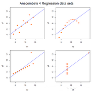
第1組數據適用于線性回歸模型，第二組使用二次模型更加合理，第三組的一個點偏離于整體數據構成的回歸直線，應該去掉。第四級做回歸是不合理的，回歸系只依賴一個點。在得到回歸方程得到各種檢驗后，還要做相關的回歸診斷。
殘差檢驗
殘差的檢驗是檢驗模型的誤差是否滿足正態性和方差齊性，最簡單直觀的方法是畫出殘差圖。觀察殘差分布情況，作出散點圖。
#20-60歲血壓與年齡分析
## (1) 回歸
rt<-read.table("d:/R-TT/book1/1_R/chap06/blood.dat", header=TRUE)
lm.sol<-lm(Y~X, data=rt); lm.sol
summary(lm.sol)

Call:
lm(formula = Y ~ X, data = rt)

Residuals:
     Min       1Q   Median       3Q      Max
-16.4786  -5.7877  -0.0784   5.6117  19.7813

Coefficients:
            Estimate Std. Error t value Pr(>|t|)    
(Intercept) 56.15693    3.99367  14.061  < 2e-16 ***
X            0.58003    0.09695   5.983 2.05e-07 ***
---
Signif. codes:  0 ‘***’ 0.001 ‘**’ 0.01 ‘*’ 0.05 ‘.’ 0.1 ‘ ’ 1

Residual standard error: 8.146 on 52 degrees of freedom
Multiple R-squared:  0.4077,    Adjusted R-squared:  0.3963
F-statistic: 35.79 on 1 and 52 DF,  p-value: 2.05e-07

## (2) 殘差圖
pre<-fitted.values(lm.sol)
 #fitted value 配適值；擬合值
res<-residuals(lm.sol)
 #計算回歸模型的殘差
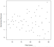
rst<-rstandard(lm.sol)
 #計算回歸模型標準化殘差
par(mai=c(0.9, 0.9, 0.2, 0.1))
plot(pre, res, xlab="Fitted Values", ylab="Residuals")
savePlot("resid-1", type="eps")

plot(pre, rst, xlab="Fitted Values",
     ylab="Standardized Residuals")
savePlot("resid-2", type="eps")

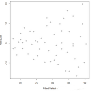
殘差
標準差


## (3) 對殘差作回歸,利用殘差絕對值與自變量（x）作回歸，其程序如下：
rt$res<-res
lm.res<-lm(abs(res)~X, data=rt); lm.res
summary(lm.res)
Call:
lm(formula = abs(res) ~ X, data = rt)

Residuals:
    Min      1Q  Median      3Q     Max
-9.7639 -2.7882 -0.1587  3.0757 10.0350

Coefficients:
            Estimate Std. Error t value Pr(>|t|)    
(Intercept) -1.54948    2.18692  -0.709  0.48179    
X            0.19817    0.05309   3.733  0.00047 ***
---
Signif. codes:  0 ‘***’ 0.001 ‘**’ 0.01 ‘*’ 0.05 ‘.’ 0.1 ‘ ’ 1

Residual standard error: 4.461 on 52 degrees of freedom
Multiple R-squared:  0.2113,    Adjusted R-squared:  0.1962
F-statistic: 13.93 on 1 and 52 DF,  p-value: 0.0004705
si= -1.5495 + 0.1982x

## (4) 計算殘差的標準差,利用方差（標準差的平方）的倒數作為樣本點的權重，這樣可以減少非齊性方差帶來的影響
s<-lm.res$coefficients[1]+lm.res$coefficients[2]*rt$X
lm.weg<-lm(Y~X, data=rt, weights=1/s^2); lm.weg
summary(lm.weg)
Call:
lm(formula = Y ~ X, data = rt, weights = 1/s^2)

Weighted Residuals:
    Min      1Q  Median      3Q     Max
-2.0230 -0.9939 -0.0327  0.9250  2.2008

Coefficients:
            Estimate Std. Error t value Pr(>|t|)    
(Intercept) 55.56577    2.52092  22.042  < 2e-16 ***
X            0.59634    0.07924   7.526 7.19e-10 ***
---
Signif. codes:  0 ‘***’ 0.001 ‘**’ 0.01 ‘*’ 0.05 ‘.’ 0.1 ‘ ’ 1

Residual standard error: 1.213 on 52 degrees of freedom
Multiple R-squared:  0.5214,    Adjusted R-squared:  0.5122
F-statistic: 56.64 on 1 and 52 DF,  p-value: 7.187e-10
修正后的回歸方程：Y = 55.5658 + 0.5963x