R語言學習筆記之聚類分析

使用k-means聚類所需的包：

factoextra

cluster #加載包

library(factoextra)

library(cluster)l 

#數據準備
使用內置的R數據集USArrests

#load the dataset

data("USArrests")

#remove any missing value (i.e, NA values for not available)

#That might be present in the data

USArrests <- na.omit(USArrests)#view the first 6 rows of the data

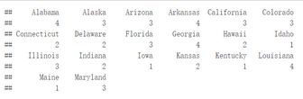
head(USArrests, n=6) 

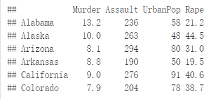
在此數據集中，列是變量，行是觀測值
在聚類之前我們可以先進行一些必要的數據檢查即數據描述性統計，如平均值、標準差等

desc_stats <- data.frame( Min=apply(USArrests, 2, min),#minimum

Med=apply(USArrests, 2, median),#median

Mean=apply(USArrests, 2, mean),#mean

SD=apply(USArrests, 2, sd),#Standard deviation

Max=apply(USArrests, 2, max)#maximum

)

desc_stats <- round(desc_stats, 1)#保留小數點后一位head(desc_stats)

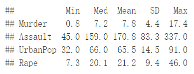
變量有很大的方差及均值時需進行標準化

df <- scale(USArrests)

#數據集群性評估
使用get_clust_tendency()計算Hopkins統計量

res <- get_clust_tendency(df, 40, graph = TRUE)

res$hopkins_stat

## [1] 0.3440875

#Visualize the dissimilarity matrix

res$plot

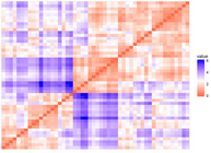
Hopkins統計量的值<0.5，表明數據是高度可聚合的。另外，從圖中也可以看出數據可聚合。

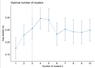
#估計聚合簇數
由于k均值聚類需要指定要生成的聚類數量，因此我們將使用函數clusGap()來計算用于估計最優聚類數。函數fviz_gap_stat()用于可視化。

set.seed(123)

## Compute the gap statistic

gap_stat <- clusGap(df, FUN = kmeans, nstart = 25, K.max = 10, B = 500)

# Plot the result

fviz_gap_stat(gap_stat)

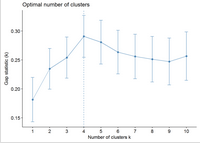
圖中顯示最佳為聚成四類（k=4）

#進行聚類

set.seed(123)

km.res <- kmeans(df, 4, nstart = 25)

head(km.res$cluster, 20)

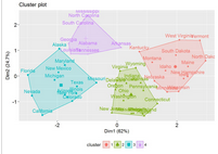
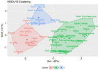
# Visualize clusters using factoextra

fviz_cluster(km.res, USArrests)

#檢查cluster silhouette圖

Recall that the silhouette measures (SiSi) how similar an object ii is to the the other objects in its own cluster versus those in the neighbor cluster. SiSi values range from 1 to - 1:

A value of SiSi close to 1 indicates that the object is well clustered. In the other words, the object ii is similar to the other objects in its group.

A value of SiSi close to -1 indicates that the object is poorly clustered, and that assignment to some other cluster would probably improve the overall results.

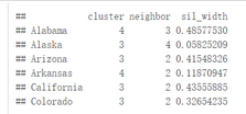
sil <- silhouette(km.res$cluster, dist(df))

rownames(sil) <- rownames(USArrests)

head(sil[, 1:3])

#Visualize

fviz_silhouette(sil)

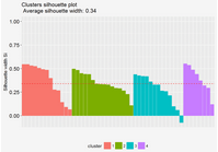
圖中可以看出有負值，可以通過函數silhouette()確定是哪個觀測值

neg_sil_index <- which(sil[, "sil_width"] < 0)

sil[neg_sil_index, , drop = FALSE]

##          cluster    neighbor     sil_width

## Missouri    3          2        -0.07318144

#eclust():增強的聚類分析

與其他聚類分析包相比，eclust()有以下優點：

簡化了聚類分析的工作流程

可以用于計算層次聚類和分區聚類

eclust()自動計算最佳聚類簇數。

自動提供Silhouette plot

可以結合ggplot2繪制優美的圖形

#使用eclust()的K均值聚類

# Compute k-means

res.km <- eclust(df, "kmeans")

# Gap statistic plot

fviz_gap_stat(res.km$gap_stat)

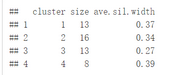
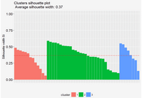
# Silhouette plotfviz_silhouette(res.km)

##    cluster size ave.sil.width

## 1     1     13      0.31

## 2     2     29      0.38

## 3     3      8      0.39

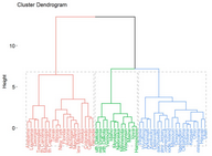
#使用eclust（）的層次聚類

# Enhanced hierarchical clustering

res.hc <- eclust(df, "hclust") # compute hclust

fviz_dend(res.hc, rect = TRUE) # dendrogam

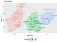
#下面的R代碼生成Silhouette plot和分層聚類散點圖。

fviz_silhouette(res.hc) # silhouette plot

##   cluster size ave.sil.width

## 1    1     19      0.26

## 2    2     19      0.28

## 3    3     12      0.43

fviz_cluster(res.hc) # scatter plot

#Infos

This analysis has been performed using R software (R version 3.3.2)