決策樹、隨機森林簡單原理和實現

一：概念

決策樹（Decision Tree）是一種簡單但是廣泛使用的分類器。通過訓練數據構建決策樹，可以高效的對未知的數據進行分類。決策數有兩大優點：1）決策樹模型可以讀性好，具有描述性，有助于人工分析；2）效率高，決策樹只需要一次構建，反復使用，每一次預測的最大計算次數不超過決策樹的深度。

看了一遍概念后，我們先從一個簡單的案例開始，如下圖我們樣本：

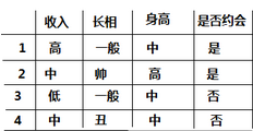
對于上面的樣本數據，根據不同特征值我們最后是選擇是否約會，我們先自定義的一個決策樹，決策樹如下圖所示：

對于上圖中的決策樹，有個疑問，就是為什么第一個選擇是“長相”這個特征，我選擇“收入”特征作為第一分類的標準可以嘛？下面我們就對構建決策樹選擇特征的問題進行討論；在考慮之前我們要先了解一下相關的數學知識：

信息熵：熵代表信息的不確定性，信息的不確定性越大，熵越大；比如“明天太陽從東方升起”這一句話代表的信息我們可以認為為0；因為太陽從東方升起是個特定的規律，我們可以把這個事件的信息熵約等于0；說白了，信息熵和事件發生的概率成反比：數學上把信息熵定義如下：H(X)＝H(P1，P2，…，Pn)＝-∑P(xi)logP(xi)

互信息：指的是兩個隨機變量之間的關聯程度，即給定一個隨機變量后，另一個隨機變量不確定性的削弱程度，因而互信息取值最小為0，意味著給定一個隨機變量對確定一另一個隨機變量沒有關系，最大取值為隨機變量的熵，意味著給定一個隨機變量，能完全消除另一個隨機變量的不確定性

現在我們就把信息熵運用到決策樹特征選擇上，對于選擇哪個特征我們按照這個規則進行“哪個特征能使信息的確定性最大我們就選擇哪個特征”；比如上圖的案例中；

第一步：假設約會去或不去的的事件為Y,其信息熵為H(Y）；

第二步：假設給定特征的條件下，其條件信息熵分別為H(Y|長相)，H(Y|收入)，H(Y|身高)

第三步：分別計算信息增益（互信息）：G(Y,長相) = I(Y,長相) = H(Y)-H(Y|長相) 、G(Y,) = I(Y,長相) = H(Y)-H(Y|長相)等

第四部：選擇信息增益最大的特征作為分類特征；因為增益信息大的特征意味著給定這個特征，能很大的消除去約會還是不約會的不確定性；

第五步：迭代選擇特征即可；

按以上就解決了決策樹的分類特征選擇問題，上面的這種方法就是ID3方法，當然還是別的方法如 C4.5;等；

二：決策樹的過擬合解決辦法

若決策樹的度過深的話會出現過擬合現象，對于決策樹的過擬合有二個方案：

1：剪枝-先剪枝和后剪紙（可以在構建決策樹的時候通過指定深度，每個葉子的樣本數來達到剪枝的作用）

2：隨機森林 --構建大量的決策樹組成森林來防止過擬合；雖然單個樹可能存在過擬合，但通過廣度的增加就會消除過擬合現象

三：隨機森林

隨機森林是一個最近比較火的算法，它有很多的優點：

在數據集上表現良好

在當前的很多數據集上，相對其他算法有著很大的優勢

它能夠處理很高維度（feature很多）的數據，并且不用做特征選擇

在訓練完后，它能夠給出哪些feature比較重要

訓練速度快

在訓練過程中，能夠檢測到feature間的互相影響

容易做成并行化方法

實現比較簡單

隨機森林顧名思義，是用隨機的方式建立一個森林，森林里面有很多的決策樹組成，隨機森林的每一棵決策樹之間是沒有關聯的。在得到森林之后，當有一個新的輸入樣本進入的時候，就讓森林中的每一棵決策樹分別進行一下判斷，看看這個樣本應該屬于哪一類（對于分類算法），然后看看哪一類被選擇最多，就預測這個樣本為那一類。

上一段決策樹代碼：

<span style="font-size:18px;"># 花萼長度、花萼寬度，花瓣長度，花瓣寬度  
    iris_feature_E = 'sepal length', 'sepal width', 'petal length', 'petal width'  
    iris_feature = u'花萼長度', u'花萼寬度', u'花瓣長度', u'花瓣寬度'  
    iris_class = 'Iris-setosa', 'Iris-versicolor', 'Iris-virginica'  
      
      
    if __name__ == "__main__":  
        mpl.rcParams['font.sans-serif'] = [u'SimHei']  
        mpl.rcParams['axes.unicode_minus'] = False  
      
        path = '..\\8.Regression\\iris.data'  # 數據文件路徑  
        data = pd.read_csv(path, header=None)  
        x = data[range(4)]  
        y = pd.Categorical(data[4]).codes  
        # 為了可視化，僅使用前兩列特征  
        x = x.iloc[:, :2]  
        x_train, x_test, y_train, y_test = train_test_split(x, y, train_size=0.7, random_state=1)  
        print y_test.shape  
      
        # 決策樹參數估計  
        # min_samples_split = 10：如果該結點包含的樣本數目大于10，則(有可能)對其分支  
        # min_samples_leaf = 10：若將某結點分支后，得到的每個子結點樣本數目都大于10，則完成分支；否則，不進行分支  
        model = DecisionTreeClassifier(criterion='entropy')  
        model.fit(x_train, y_train)  
        y_test_hat = model.predict(x_test)      # 測試數據  
      
        # 保存  
        # dot -Tpng my.dot -o my.png  
        # 1、輸出  
        with open('iris.dot', 'w') as f:  
            tree.export_graphviz(model, out_file=f)  
        # 2、給定文件名  
        # tree.export_graphviz(model, out_file='iris1.dot')  
        # 3、輸出為pdf格式  
        dot_data = tree.export_graphviz(model, out_file=None, feature_names=iris_feature_E, class_names=iris_class,  
                                        filled=True, rounded=True, special_characters=True)  
        graph = pydotplus.graph_from_dot_data(dot_data)  
        graph.write_pdf('iris.pdf')  
        f = open('iris.png', 'wb')  
        f.write(graph.create_png())  
        f.close()  
      
        # 畫圖  
        N, M = 50, 50  # 橫縱各采樣多少個值  
        x1_min, x2_min = x.min()  
        x1_max, x2_max = x.max()  
        t1 = np.linspace(x1_min, x1_max, N)  
        t2 = np.linspace(x2_min, x2_max, M)  
        x1, x2 = np.meshgrid(t1, t2)  # 生成網格采樣點  
        x_show = np.stack((x1.flat, x2.flat), axis=1)  # 測試點  
        print x_show.shape  
      
        # # 無意義，只是為了湊另外兩個維度  
        # # 打開該注釋前，確保注釋掉x = x[:, :2]  
        # x3 = np.ones(x1.size) * np.average(x[:, 2])  
        # x4 = np.ones(x1.size) * np.average(x[:, 3])  
        # x_test = np.stack((x1.flat, x2.flat, x3, x4), axis=1)  # 測試點  
      
        cm_light = mpl.colors.ListedColormap(['#A0FFA0', '#FFA0A0', '#A0A0FF'])  
        cm_dark = mpl.colors.ListedColormap(['g', 'r', 'b'])  
        y_show_hat = model.predict(x_show)  # 預測值  
        print y_show_hat.shape  
        print y_show_hat  
        y_show_hat = y_show_hat.reshape(x1.shape)  # 使之與輸入的形狀相同  
        print y_show_hat  
        plt.figure(facecolor='w')  
        plt.pcolormesh(x1, x2, y_show_hat, cmap=cm_light)  # 預測值的顯示  
        plt.scatter(x_test[0], x_test[1], c=y_test.ravel(), edgecolors='k', s=150, zorder=10, cmap=cm_dark, marker='*')  # 測試數據  
        plt.scatter(x[0], x[1], c=y.ravel(), edgecolors='k', s=40, cmap=cm_dark)  # 全部數據  
        plt.xlabel(iris_feature[0], fontsize=15)  
        plt.ylabel(iris_feature[1], fontsize=15)  
        plt.xlim(x1_min, x1_max)  
        plt.ylim(x2_min, x2_max)  
        plt.grid(True)  
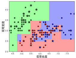
        plt.title(u'鳶尾花數據的決策樹分類', fontsize=17)  
        plt.show()  
      
    </span>  

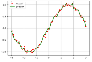
以上就是決策樹做分類，但決策樹也可以用來做回歸，不說直接上代碼：
[python] view plain copy

    <span style="font-size:18px;">if __name__ == "__main__":  
        N =100  
        x = np.random.rand(N) *6 -3  
        x.sort()  
        y = np.sin(x) + np.random.randn(N) *0.05  
        x = x.reshape(-1,1)  
        print x  
        dt = DecisionTreeRegressor(criterion='mse',max_depth=9)  
        dt.fit(x,y)  
        x_test = np.linspace(-3,3,50).reshape(-1,1)  
        y_hat = dt.predict(x_test)  
      
        plt.plot(x,y,'r*',ms =5,label='Actual')  
        plt.plot(x_test,y_hat,'g-',linewidth=2,label='predict')  
        plt.legend(loc ='upper left')  
        plt.grid()  
        plt.show()  
      
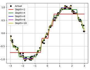
        #比較決策樹的深度影響  
        depth =[2,4,6,8,10]  
        clr = 'rgbmy'  
        dtr = DecisionTreeRegressor(criterion='mse')  
        plt.plot(x,y,'ko',ms=6,label='Actual')  
        x_test = np.linspace(-3,3,50).reshape(-1,1)  
        for d,c in zip(depth,clr):  
            dtr.set_params(max_depth=d)  
            dtr.fit(x,y)  
            y_hat = dtr.predict(x_test)  
            plt.plot(x_test,y_hat,'-',color=c,linewidth =2,label='Depth=%d' % d)  
        plt.legend(loc='upper left')  
        plt.grid(b =True)  
        plt.show()</span>  

不同深度對回歸的 影響如下圖：

下面上個隨機森林代碼
[python] view plain copy
    mpl.rcParams['font.sans-serif'] = [u'SimHei']  # 黑體 FangSong/KaiTi  
    mpl.rcParams['axes.unicode_minus'] = False  
      
    path = 'iris.data'  # 數據文件路徑  
    data = pd.read_csv(path, header=None)  
    x_prime = data[range(4)]  
    y = pd.Categorical(data[4]).codes  
    feature_pairs = [[0, 1]]  
    plt.figure(figsize=(10,9),facecolor='#FFFFFF')  
    for i,pair in enumerate(feature_pairs):  
        x = x_prime[pair]  
        clf = RandomForestClassifier(n_estimators=200,criterion='entropy',max_depth=3)  
        clf.fit(x,y.ravel())  
        N, M =50,50  
        x1_min,x2_min = x.min()  
        x1_max,x2_max = x.max()  
        t1 = np.linspace(x1_min,x1_max, N)  
        t2 = np.linspace(x2_min,x2_max, M)  
        x1,x2 = np.meshgrid(t1,t2)  
        x_test = np.stack((x1.flat,x2.flat),axis =1)  
        y_hat = clf.predict(x)  
        y = y.reshape(-1)  
        c = np.count_nonzero(y_hat == y)  
        print '特征：',iris_feature[pair[0]],'+',iris_feature[pair[1]]  
        print '\t 預測正確數目：',c  
        cm_light = mpl.colors.ListedColormap(['#A0FFA0', '#FFA0A0', '#A0A0FF'])  
        cm_dark = mpl.colors.ListedColormap(['g', 'r', 'b'])  
        y_hat = clf.predict(x_test)  
        y_hat = y_hat.reshape(x1.shape)  
        plt.pcolormesh(x1,x2,y_hat,cmap =cm_light)  
        plt.scatter(x[pair[0]],x[pair[1]],c=y,edgecolors='k',cmap=cm_dark)  
        plt.xlabel(iris_feature[pair[0]],fontsize=12)  
        plt.ylabel(iris_feature[pair[1]], fontsize=14)  
        plt.xlim(x1_min, x1_max)  
        plt.ylim(x2_min, x2_max)  
        plt.grid()  
    plt.tight_layout(2.5)  
    plt.subplots_adjust(top=0.92)  
    plt.suptitle(u'隨機森林對鳶尾花數據的兩特征組合的分類結果', fontsize=18)  
    plt.show()